MathBits.com Table of Contents 1

Graphing Residuals

(What is a residual?  See "Residuals and Least Squares".)

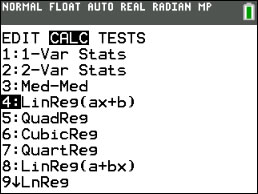
The graphing calculator uses a least squares regression equation to determine regression models.  When regression models are computed, residuals are automatically stored in a list called RESID. 
  
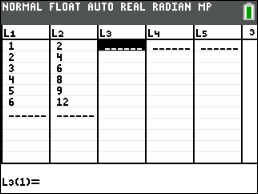
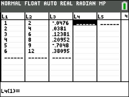
If you want to see the RESID list, in the column list section of the calculator, you can place the values in L3 (for example).  Go to STAT and choose EDIT.  Place the cursor on the heading for L3.  Press LIST (2nd STAT) and choose #7 RESID.  Press ENTER.  The residual values are now in L3 for easy viewing.


Consider this set of data (which is “almost” a perfect linear equation)

2  3  4

5  6

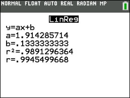
If the data had been a perfect linear equation, you would have:

7  8  9

10  11  12

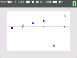
After adjusting the window, just hit GRAPH (not Zoom).

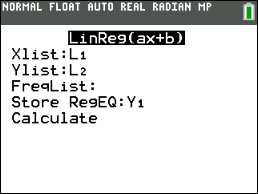
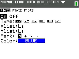
Step-by-step Instructions for Producing a Residual Plot:

1. Store your data in lists.
Enter the x-values in
L1 and the y-values in L2.
rprocess1
2. Perform a linear regression.

STAT, arrow right to CALC, choose either 4:LinReg(ax+b) or 8:LinReg(a+bx)

rprocess2
3. Store the regression equation in Y1.rprocess3 rprocess4
4. Go to the top of L3 and press ENTER.
The cursor is now flashing at the bottom of the screen after L3 =.
Type in L2 - Y1(L1).
The Y1(L1) will calculate the regression y-values by placing each x-value into your regression equation.
OR
Go to the top of L3 and press ENTER.
Press LIST (2nd STAT) and choose #7 RESID.  Press ENTER.
rprocess5
5. Go to the STAT PLOT menu (2nd Y=).
Choose Plot1, hit ENTER.
Turn the Plot ON (by hitting ENTER).
Arrow down to Type: choose the first option (scatter plot).
Make XList: L1 (the x-values)
Make YList: L3 (the residuals)


rprocess6
6. Go to ZOOM.
Choose ZOOM 9:ZoomStat
You should see your Residual Plot.
rprocess7

14
Finding Your Way Around TABLE of  CONTENTS